Model Building
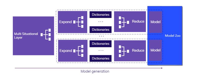
TIM strives to follow all best practices in time-series modeling to achieve the best possible accuracy as fast as possible. The architectural design of the model building phase of the TIM engine is illustrated in the schema below.
Schema

This schema's main components and their specifics are discussed in the following sections. How the model building phase fits into the overall TIM Forecasting solution can be found in the Structure section.
The multi-situational layer
When building a model, TIM tries to recognize all situations that might require (or benefit from) a specific model. A situation in this context is a combination of the time of forecasting, the forecasting horizon and the data availability. Usually, many different situations occur. TIM creates a separate model for each situation optimized to the situation's conditions, and then combines all of these models into one Model Zoo. Every time TIM is asked to make a forecast, the current situation is automatically recognized, the appropriateness of each model is assessed, all required models are built (depending on the type of job) and finally, the forecast is produced.
This property enables the creation of very simple models for straightforward situations - such as solar production at night, for example - and more complex models for more challenging situations. In other words, TIM can include necessary complexity in certain situations while eliminating redundant complexity in other situations. As a lot of focus is placed on TIM's fast forecasting capabilities, it is important that TIM can recognize how these situations differ from each other. TIM can intelligently exploit similarities between models during model building.
TIM's multi-situational layer runs this optimization of all individual models.
Different situations
Three qualities distinguish different situations from each other:
- The distance between the timestamp of the desired forecast and the last available target observation: This relates back to the position of the timestamp in the desired forecasting horizon. In general, TIM creates a separate model for each point in the forecasting horizon. This is because it is more challenging to forecast further into the future and thus models built to forecast over a different distance should be able to vary in their complexity.
- The specific time of day of the timestamp of the desired forecast: Some datasets exhibit a property called daily cycle. This means there is a visible periodicity within a day influenced by socio-economic or other factors repeating day after day - in other words, a daily seasonality. It is often more difficult to forecast something happening at noon than during the night. In such cases, TIM distinguishes different times of the day and creates a separate model for each time. The detection of a daily cycle is done automatically, but can also be set manually.
- The distance between the timestamp of the desired forecast and the last available timestamps of every predictor: One of the essential features extracted from the data when dealing with time series are offsets (lags) of the predictors. The available offsets often differ from time to time because of irregularities in the data gathering processes. TIM tries to exploit the predictive power of the most recent available data records and therefore distinguishes between a situation where, for example, a -24 offset of a predictor is available and a situation where a -22 offset of the predictor is available. It's often worth building a new model if you can use a closer offset of a predictor than the one a previously built model used. Vice versa, it is necessary to build a new model if an offset of a predictor that a previously built model relied on is no longer available.

Situations versus models
After TIM is given a forecasting task, it first recognizes all situations (as described above) to be addressed. Then, for rebuild-model job types, it looks at all situations covered by the models in the attached Model Zoo. The situations that lack models are sent to the model building process, and new models are generated to cover them. Finally, the old Model Zoo is merged with the new models and returned for further use. This enables users to significantly shorten the forecasting time required in production by interpreting already built models instead of building the entire Model Zoo from scratch. The whole rebuilding process can also be configured to better suit the needs of any particular application.
Expansion
TIM goes through all predictors included in the dataset to differentiate the important ones from those that do not contribute to the final results. In the expansion process, TIM creates many new features from the original predictors to enhance the final model's performance. This is done through a set of common transformations called features. If some of the features do not contribute to a better model performance, TIM can recognize this without compromizing on accuracy.
Reduction
The previously discussed process of expansion creates many new features. It is not optimal to retain all of these new features in the final model(s), as many will likely be highly correlated. Having highly correlated features in a model makes the highly unstable: a slight change in a feature could result in a structural change of the whole model, since the model's results are influenced by many similar features (highly correlated with the one that initially changed). This is not desirable. Therefore, only the most important subset of features will be retained for the final model, eliminating the high correlation among various features.
Increasing model stability by eliminating inner correlation is similar to fighting a phenomenon called overfitting.
Choosing a smaller subset of variables or features - i.e. the reduction process - is a widely researched topic; algorithms like LASSO, PCA and forward regression are all well known to the public. TIM uses a similar technique that heavily relies on a geometrical perspective and incorporates a tweaked Bayesian Information Criterion.